The 34 DAX Functions I Use To Answer 95% Of Business Problems

With over 250 DAX functions available, how do you know which ones you should learn?

Jan 28, 2024

With over 250 DAX functions available, how do you know which ones you should learn?

Simple answer: without experience, you don't. This article will address that pain 💊 by walking you through a list of 34 handpicked functions that I have personally used to solve real-life problems. I have to warn you, though, as a side effect, you might end up saving years' worth of effort and skip all the painful trial and error.

All the functions will be accompanied by a short story explaining the logic behind why that specific function made it to the list.

What you should know to get most out of this article

Let me begin by testing how comfortable you are with DAX by quickly firing off a few terms.

Scalar value, table, iterator, aggregator, data model, relationship. How did those words make you feel? If they caused any anxiety, I suggest you first read my previous article to learn some fundamental DAX concepts. If all of the terms sounded familiar, you’re cleared to move on 🫡.

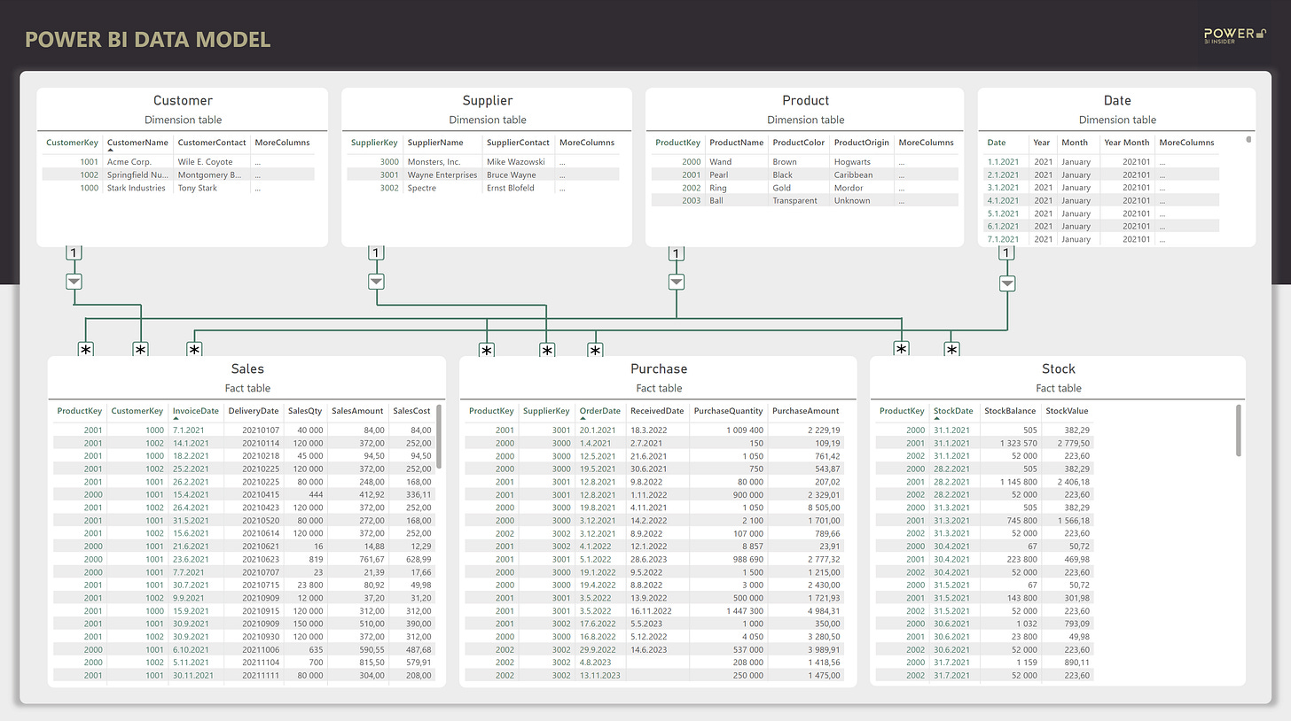
As you know, it will be impossible to understand DAX without knowing how the data model on the background looks like, so please start by memorizing 😳 the below picture.

Ok, time dive in. Don’t be fooled by the first few simple examples. There’s some advanced DAX tricks 🔞 waiting for you in the later examples.

First things first, I’d like to know how much money are we making?

Let’s start with some basic aggregator functions 👶🍼 to get warmed up.

SUM, MIN, MAX, and AVERAGE are the basic set of functions you should use when you need a simple aggregation AND don’t need row by row calculation. To compute [Sales Amount] we can simply use the SUM function to aggregate the ‘Sales’SalesAmount column. Following similar logic it’s possible to add other measures like [Sales Quantity] or [Purchase Value].

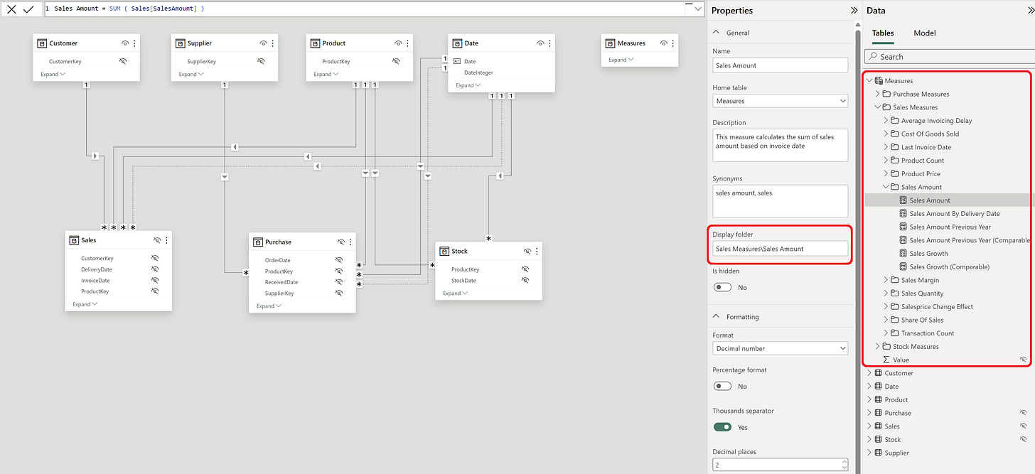
To make life easier in future, I will store all measures in a dedicated table that has a logical easy to follow structure.

Great, we have some sales, what about the count of sales transactions?

Continuing with the basics, COUNTROWS is another useful function, but you might not know about it if you're new to DAX.

COUNTROWS simply counts how many rows are in the table (not a column) you provide it, and returns a whole number (or have you ever heard of a table that contains 10,5 rows? 🤔). Use it whenever you need to know the total row count of a table (duplicates included) — [Count Of Sales Transactions] is a perfect example of this.

With the measure created, a quick reminder to always give your DAX measures a descriptive name, even if it means that the name becomes longer. It’s possible to rename the measure in the visualization as I’ve done below with # Transactions.

Example: renamed Count Of Sales Transactions

I’m starting to form a picture here, but how many products are we selling?

It looks like COUNTROWS has brought it’s cousin to the party 🥳.

Let's give a warm welcome to DISTINCTCOUNT! While COUNTROWS counts the rows in a table, DISTINCTCOUNT counts the unique values in a column. It might be pretty obvious you should use it whenever you need to count unique values instead of all values, like now when we compute the distinct count of ProductKeys in ‘Sales’ table.

Besides giving measures descriptive names, give them also a common sense description in the model view so that also business users understand what your measure does.

Since we’re on the topic of unique VALUES here, it makes sense to mention VALUES function.

VALUES is a function that returns a one column table containing unique values of a column you provide it. You will need this type of table quite often. *It is also possible to provide a whole table to VALUES, instead of a single column, but from my opinion that is a more rare use case (if you need more details, check it from here).

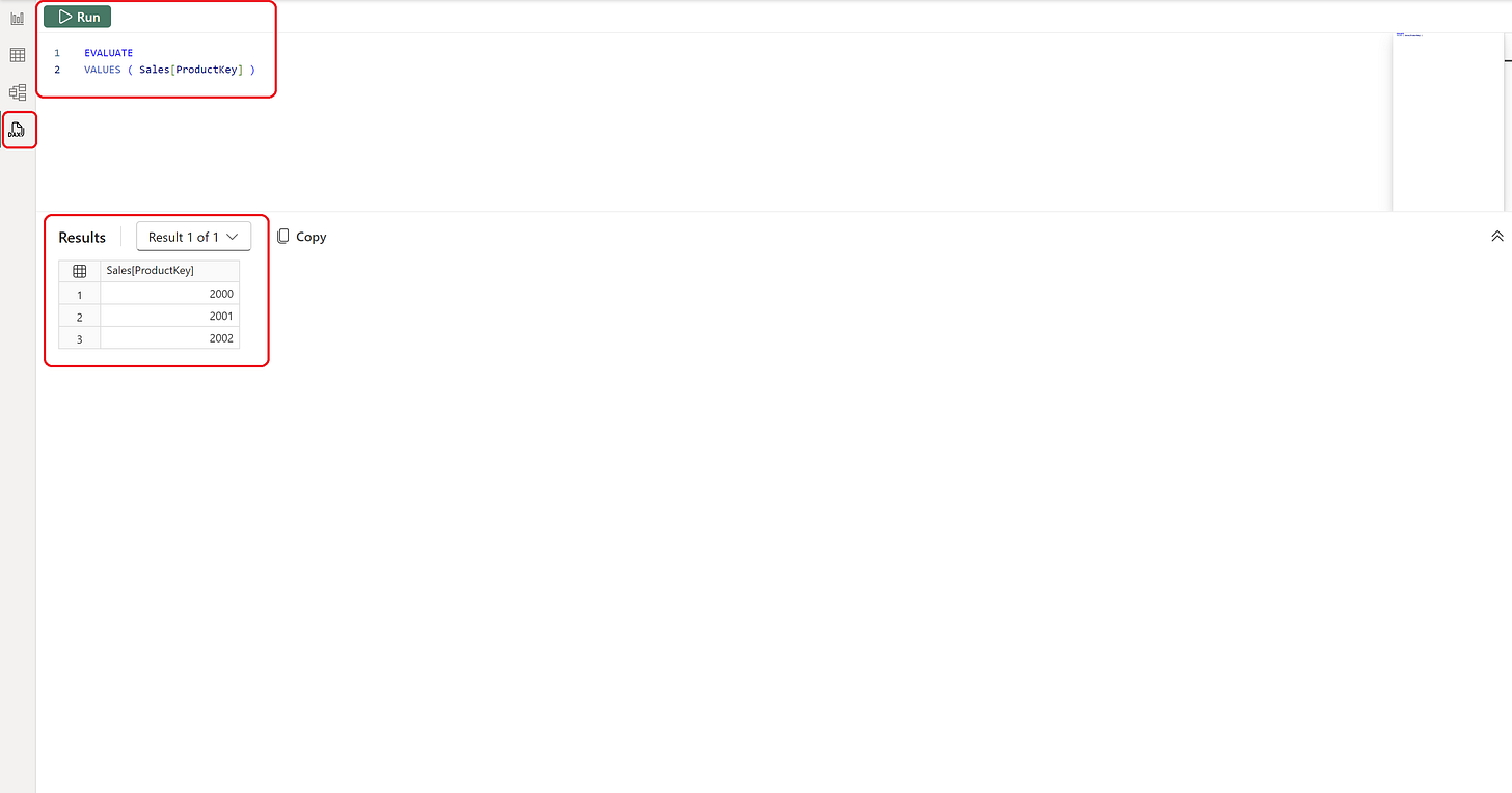
Because VALUES returns a table, It’s not possible to display the result in a visualization. But why don’t we test the brand new Query View in Power BI Desktop to see what a table of unique ProductKeys looks like.

For now, this is enough unique values, but remember what VALUES does, as we will be using it again later in this article.

Is it possible to also see what is the average sales price for each product?

Of course! Because I’m a big supporter of reusability, lets try to use the measures created so far.

To compute average sales price, we need to divide [Total Sales] with [Sales Transaction Count] using (this is going to shock you 😲) the DIVIDE function. DIVIDE is a handy function because with it, you can specify what value should be returned in case of a division by zero error. Enough years in Excel really teaches you to hate that bloody #DIV/0! 🤬. If you don’t need division by zero handling, the classic division “/” sign provides a better performance.

You can also use DIVIDE to return a blank value instead of a zero using this syntax: _YourValue * DIVIDE ( _YourValue, _YourValue ). If you decide to use it, pair it with a variable so that you don’t have to compute the same value three times.

Before we continue ✋, remember to always set the format to your measures. There is nothing more unprofessional looking than a random number of decimals points or a missing thousand separator 😤.

Example: DIVIDE function & measure format settings

Sorry, but that average sales price does not make any sense on customer and total level

But you probably already noticed that, IF you’re actually focusing in reading this article 🧐

The average sales price on total level is totally meaningless because when you divide sales of multiple products with sales quantity of multiple products, the result does not mean anything. Let’s fix that using IF and HASONEVALUE functions. IF is a great function to use whenever you have only one logical rule to check, and paired with HASONEVALUE we can easily check if we have just one product in the current filter context.

Speaking of this technique, SELECTEDVALUE is another useful function that performs exactly the same IF HASONEVALUE check, and if there only is one value, returns that value. In case of many values you can define which value should be returned, if any. This is how it all looks like:

It could be nice to also label the average sales price as cheap or expensive

We could do that by writing multiple nested IF statements, but there’s also a better way to do it, using SWITCH function.

SWITCH belongs to the family of logical functions, but contrary to IF, it can check multiple 🤹‍♂️ logical rules and returns the value when the logical check is TRUE. Take a look on the picture below to see how easy it is to assign products into three different price tiers.

If you're wondering about the reason for using the _underscore sign in front of variable names, it’s best practice so that you can clearly distinguish variables. It also makes writing DAX easier because intellisense will suggest you only variables when you start by typing _.

Going back to sales, I forgot to ask if it’s possible to display share of sales % between customers?

Stop asking if it’s possible already, anything is possible using DAX! 🔥

We just need to ask help from the superhero of DAX 🦸‍♂️, CALCULATE function. With CALCULATE it’s possible to add, remove, or change the filters that affect your calculation. On top of that CALCULATE performs context transition, but that really deserves an article of it’s own. But back to the story now.. Let’s use CALCULATE paired with it’s buddy REMOVEFILTERS to calculate sales for all customer, so that we can compare it with sales to currently filtered customer. It’s good to understand REMOVEFILTERS is only a sidekick for CALCULATE, it does not return value of any kind by itself. If you need a table with all filters removed, you should use ALL function for the job.

If you’ve already stumbled into CALCULATETABLE function somewhere, it’s good to know the only difference to CALCULATE is that it returns a table as the result instead of a single value.

Example: CALCULATE & REMOVEFILTERS functions

Hey hey hey, wait a sec, why is that share of sales not 100% on total level?

Good question! It looks like I had a filter on the page to only show two customers, and by using REMOVEFILTERS we calculated the sales for every single customer in the whole data model.

If you want the share of sales % of what you see, you should use ALLSELECTED function paired with CALCULATE. (In reality, ALLSELECTED does complex things behind the scenes, restoring the last shadow filter context 👻, but that’s seasoned DAX warrior 🪖🎖️ stuff). What you need to know is that you can use ALLSELECTED with peace of mind in to compute “all you can see 👀” total.

If for some reason you manage to get a punch 🥊 in the face from ALLSELECTED, go visit this page and the related articles.

Next I’d like to see the sales growth compared to previous year, since if you’re not growing, you’re dying

Time to introduce our first time intelligence function ⌛️, DATEADD, my personal favorite thanks to it’s versatility.

Now, for time intelligence functions to work properly, always remember to use a proper Date table in your data model! After you have checked that box you can use DATEADD to start time travelling 👽 in days, months, quarters, or years (but not in weeks). DATEADD returns a single column table of dates shifted backwards or forward in time, that you can then use as a filter in CALCULATE to compute the sales of previous year, and finally the growth of sales.

If you prefer, you can use also SAMEPERIODLASTYEAR function instead of DATEADD - 1 YEAR.

Is that really correct? The growth is negative, but I thought we’ve had a good start to year in sales?

Aha! It’s because I have a relative date filter “This year” (1.1.2024 - 31.12.2024) on the page.

DATEADD moves this entire filter one year back (1.1.2023 - 31.12.2023), and because I only have sales in January 2024 so far, I end up comparing it against the full year sales of 2023. Let me just quickly fix this by changing the relative date filter to “this year so far”. But… But where is it? Microsoft? Anyone? No option for that? Seriously?.. Ok, let’s do it with DAX then 🤷‍♂️.

We can do this by using KEEPFILTERS function. KEEPFILTERS is another function that can be only used inside CALCULATE and it doesn’t exactly return a value or table, it changes filter behavior. The default behavior of CALCULATE is to override filters, so if we would just say ‘Date’Date ≤ _LastSalesDate, we would completely override the relative date filter. We don’t want that. However, by using KEEPFILTERS it’s possible to add new filters and KEEP the existing filters in case they also pass the new filter.

So, to form a table of comparable dates for both years, let’s wrap the the ‘Date’Date ≤ _LastSalesDate into KEEPFILTERS. This will keep the dates coming from the relative date filter but only if those days are on or before the last invoice date.

Then we will simply use this table of comparable dates as a filter to compute a revised, actually comparable version of the existing [Sales Amount Previous Year] measure.

If you know someone that might get value out of this article, why not share it?

That got me wondering, how much of that sales growth is coming from price increases to customers?

To compute the effect of price increases, the very first thing we need to know is which products are sold to which customers.

On this problem, we turn to SUMMARIZE function. SUMMARIZE groups a table based on the columns you provide it, and returns a summarized version of that table as the result. Again, because SUMMARIZE returns a table the only way to easily display how the result works is to show it with the Query View. Here’s how sales table grouped by customer and product looks like:

But how do you use this table to compute price increases?

Time to meet the X relatives of the basic aggregator functions: SUMX, MAXX, MINX, AVERAGEX. Don’t ask me where the X ending comes from (maybe someone wiser than me can leave a comment about that). All X functions iterate a table you provide it row by row, and perform a sum, min, max or average of the row level results depending on which X function you use.

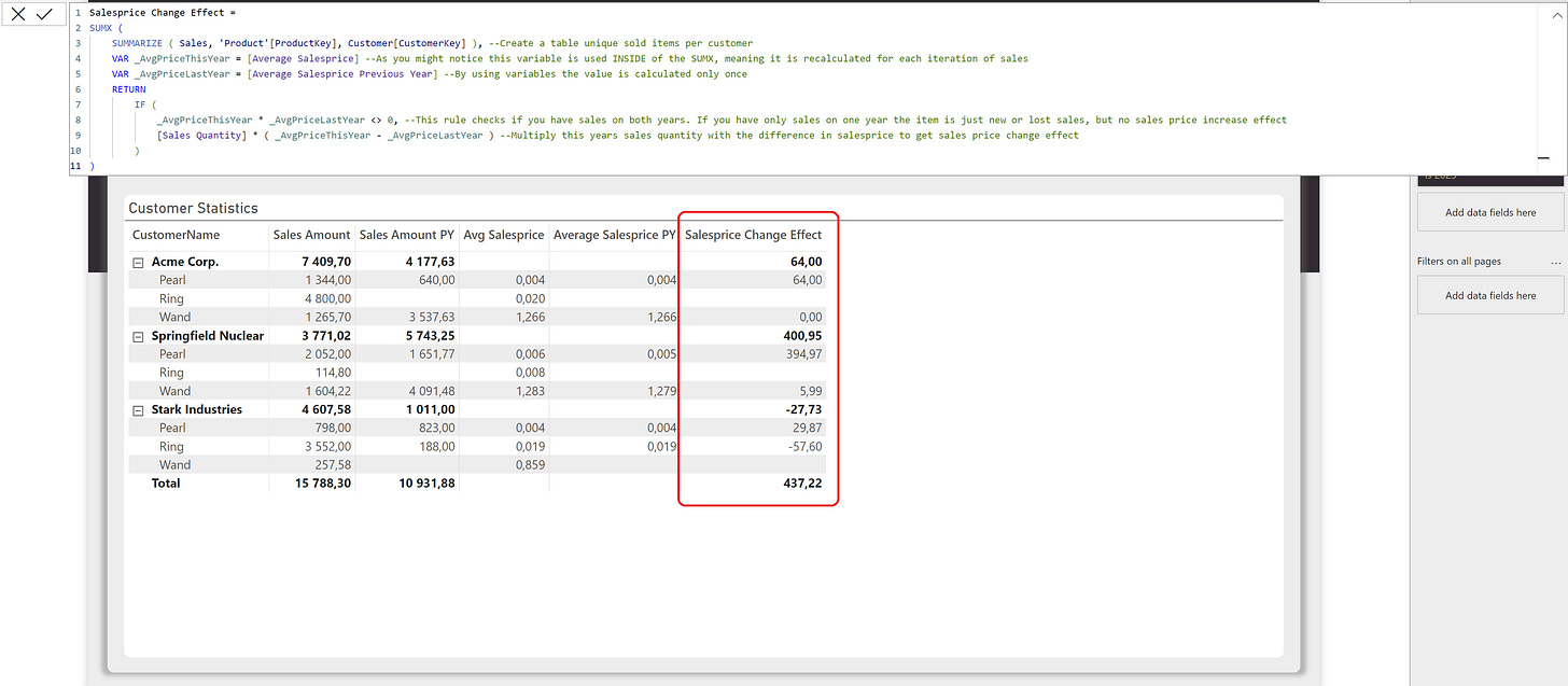
In our example, we’re going to use SUMX because is sounds cool 😎. Just kidding, we use it because we need a sum of price increases. SUMX will iterate our table of customer product combinations row by row, compare the difference in average sales price between this year and last year, multiply the difference with sales quantity, and finally sum the result.

BOOM 💣, just like that you know exactly the effect of price increases to your business.

One customer has a negative price increase. Please tell me we are not selling any products with a low sales margin %?

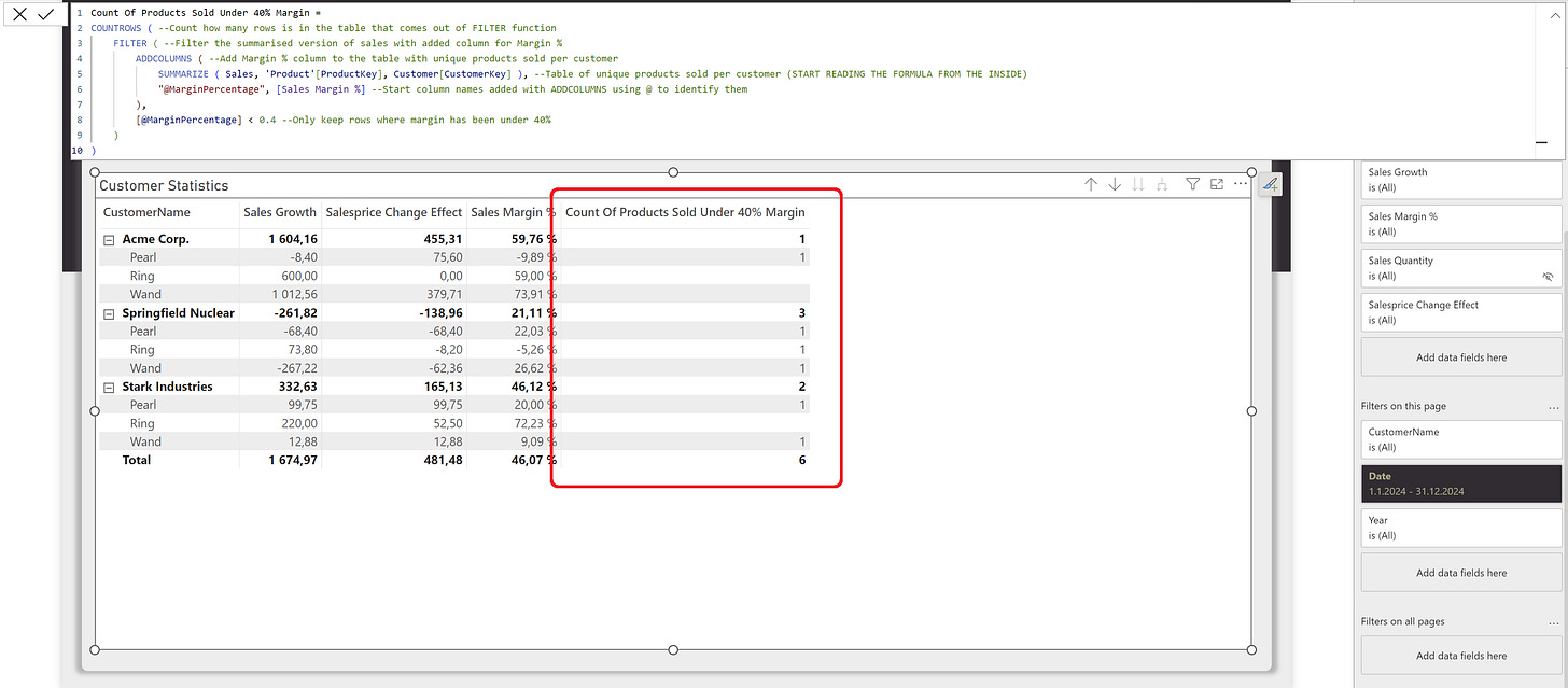
To be able to answer that question, we need to compute the count of products that have been sold under a specified sales margin %.

I suggest we start to build the solution to this problem from the inside out. Again, as a base we need a table of sold products per customer (you already know how to do this thanks to previous example). But we also need to add a column to know the sales margin % for each customer and product combination. To do that we will use ADDCOLUMNS function (Finally a function name that clearly describes what it does 😌). As the name suggests, ADDCOLUMNS adds new columns to the table you provide it by iterating row by row.

Here’s how the result of ADDCOLUMNS looks like in Query View:

As you’ve now seen, many times the power of DAX comes to play when using multiple functions together. So how about we add another layer to this calculation.

We now have a table of all customer and product combinations sold, enriched with the sales margin %. Next we need to find a way to filter this table so that only the rows with low sales margin % remain. To do it, we will use 🥁…. the FILTER function! What a shocker! Now.. what is considered a low margin varies quite much on the industry, but in our business of selling magic wands 🪄 and crystal balls 🔮, let’s say our treshold for low sales margin is 40%.

Finally, we need to know how many rows remain in the final table. For that we ask a favor from our old friend and wrap the whole thing inside COUNTROWS.

Example: using multiple functions together

Clearly we need to work bit more on our pricing, but are we at least invoicing our customers right after delivery?

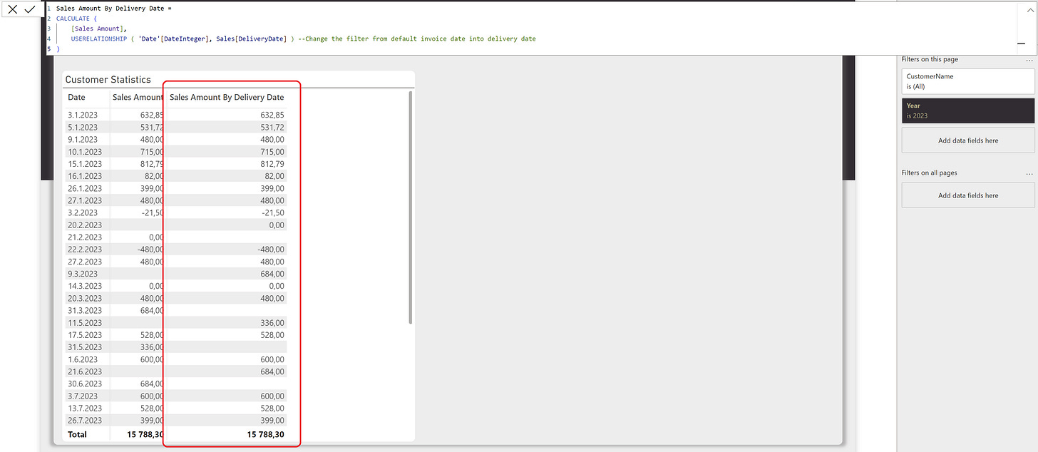
You know, the data model behind DAX is quite a Casanova 🤵‍♂️, and it’s not uncommon to see multiple relationships between two tables.

This data model is no exception, because the ‘Sales’ table has two relationship withs ‘Date’ table using invoice date and delivery date. Leveraging that fact, it should be simple to just create a measure for Sales Amount based on delivery date. In fact, it is, we just need to use the USERELATIONSHIP function inside CALCULATE function to activate the relationship between date and sales delivery date. Then, We can then easily display [Sales Amount By Delivery Date] side by side with the [Sales Amount] by invoice date.

Aaaand of course it looks like we’re not invoicing on the date of delivery (should have guessed that by now🤦‍♂️).

Since there seems to be a gap, how long is the average invoicing delay after delivery?

OK, this is going to be easy.

We will just use the DATEDIFF, which compares the difference between two dates, delivery date and invoicedate. To get correct average, we will perform the calculation row by row using AVERAGEX.

The only thing I forgot was the fact that delivery date is stored as whole number in ‘Sales’ table because I made a call to not break query folding. Gotta love the decision to store dates as whole numbers in the database ❤️. Well, it seems like we have some DAX work ahead of us again because DATEDIFF does not like to play with whole numbers. To work around this issue we will resort to the help text functions LEFT, MID, and RIGHT to extract the year, month, and day from the whole number, and convert that into a proper date using DATE function.

Now we can finally see the average delay of invoicing. And that ladies and gentleman, is leaving money on the table 💵 with todays interest rates.

Perhaps we can also take a look how much stock we have for each customer?

Of course, this will be simply a sum of stock value.

We just need to pay attention and realize that the ‘Stock’ table is different compared to ‘Sales’ and ‘Purchase’ tables. The difference is that the ‘Stock’ table contains monthly snapshots which cannot be aggregated. Instead we need to compute the stock value for last selected snapshot. This can be easily done using functions we’ve already used in this article: MAX, SUM and CALCULATE.

But wait, why is the stock value the same for all customers and items?

Well, now that you said it, I can see there is no relationship between the ‘Customer’ and ‘Stock’ table. When I filter the ‘Customer’ table, it only filters the ‘Sales’ table, not ‘Stock’ 🤔. I might change the relationship between ‘Sales’ and ‘Product’ to be bi-directional to fix this, but because a wise man 🧙‍♂️ once told me to never do it, I wont. Fortunately, there isn’t a problem that can’t be solved with DAX💡!

Whenever you run into complex relationship issues, what do you do? You call in Dr. Phil 👴🏻! The DAX equivalent of that is the TREATAS function. TREATAS allows you to “teleport” filters from one table to another, no matter how the relationships between the tables have been set up. So, to fix this issue, we will first create a table of items that have been sold to a specific customer (from ‘Sales’ table), and then filter the ‘Product’ table using this virtual magic table. ‘Product’ table will then naturally filter the ‘Stock’ table following the regular relationship.

Ok, it looks like we’re not quite there yet.

While our formula technically works, unfortunately each product has been sold to each customer, totaling to a result that doesn’t really tell much. No bueno 🙅‍♂️! On top of that, the stock value on total level is now incorrect because one of the products has not been sold to any customers ever in history. Time to put our DAX Gi 🥋 on and finally submit this formula.

To fix the first issue, we want to distribute the stock value based on which customer has bought most of it in history. To do it, we will iterate all products and multiply the [Stock Value Customer] measure with another already created measure [Share Of Sales Amount % All History]. To fix the second issue, we will use the ISFILTERED function to check if there is a filter on ‘Customer’ table, and if not, return the original [Stock Value] measure that also displays the value for the products that have not been sold any customer.

Bulls eye 🎯, finally the formula works as we would like.

That is magic, the last thing I would like to know is how long does it take to turn the inventory one time?

Gotta give you a fist bump 🤜🤛 for making it all the way to the last example of this lengthy article (maybe I should turn this into a book 🤔).

To compute the classic stock measure [Days Inventory Outstanding], we reach out for another amazing time intelligence function, DATESINPERIOD. It’s a great function whenever you need to create a table of consecutive dates starting from a specified date. In our example we create a table of previous 12 months dates starting from the last selected date in the report. Then we use that table as a filter in CALCULATE to compute both cost of goods solds and average inventory value from previous 12 months.

With that we can see that it takes on average 302 days to turn the inventory once, bit too slow if you ask me.

That concludes the article. If you managed to follow each example, I guarantee you will be well on your way to becoming a true DAX Ninja 🥷🏿!

Power BI Insider

Discussion about this post